In my blog dated September 3, 2021, I introduced a very simple formula to dispel the fears of the plummeting sales under COVID-19. The formula is as follows.
$$x_{t}=αx_{t-1}+µ+ε_{t}\tag{1}$$
where xt is the sales at time t, xt-1 is the previous sales, α is the sales coefficient, µ is a constant, and εt is the error term. This simple equation tells us that the sales that dropped due to COVID-19 will always return to their original state. COVID-19 was expressed by giving a large negative value to εt, but let’s examine the opposite case, which is positive.
First, let’s check if the stimulus is in the normal range.
Fig. 1
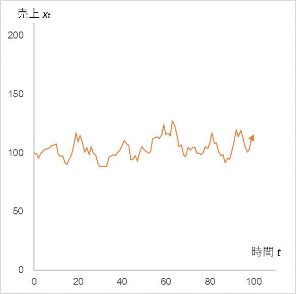
Time series change of sales xt (initial value = 100) calculated by substituting εt, which follows a normal distribution
with α = 0.9, µ = 10, mean = 0, and standard deviation = 5, into equation (1)
The vertical motion continues around the initial value of 100. Now, replace εt with +50, +40, +30, and +20 for t=10 to 13.
Fig. 2
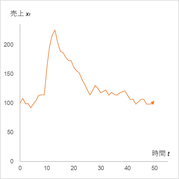
Time series change of sales xt (initial value = 100) calculated by substituting εt
with α = 0.9, µ = 10, mean = 0, and standard deviation = 5 into equation (1)
(Note that εt is +50 at t=10, +40 at t=11, +30 at t=12, and +20 at t=13.)
Sales in the period t=10 to 13 jump greatly due to the positive stimulus, but quickly return to the original jagged state again. This is the reason why even if sales increase rapidly due to advertising activities, they immediately return to the previous level when the activities are stopped. Now, what about the case where we continue the advertising activities, let’s increase the average of εt from 0 to 10 after t=14.
Fig. 3
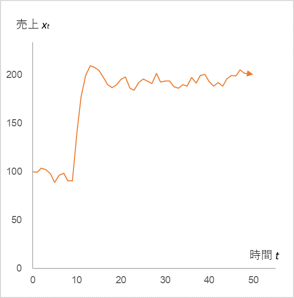
In Fig. 2, the time series change in sales xt when the mean of εt after t=14 is increased from 0 to 10 (the standard deviation remains 5).
Indeed, sales have remained high and sustained. Continuity is power. This explains why we see the same manufacturer’s commercials on TV over and over again, and why the companies exhibiting at trade shows are always the same.
The reason why we return to the same level again even after stimulation can be understood by expanding equation (1) as follows.
$$x_{0}$$
$$x_{1}=αx_{0}+µ+ε_{1}$$
$$x_{2}=αx_{1}+µ+ε_{2}=α(αx_{0}+µ+ε_{1})+µ+ε_{2}=α^2x_{0}+µ(1+α)+(αε_{1}+ε_{2})$$
$$x_{3}=αx_{2}+µ+ε_{3}=α(α^2x_{0}+αµ+αε_{1}+µ+ε_{2})+µε_{3}=α^3x_{0}+µ(1+α+α^2)+(α^2ε_{1}+αε_{2}+ε_{3})$$
・
・
・
$$x_{t}=αx_{t-1}+µ+ε_{t}=α^tx_{0}+µ(1+α+α^2+α^3+ ・・・+α^t)+(α^{t-1}ε_{1}+α^{t-2}ε_{2}+α^{t-3}ε_{3}+・・・+ε_{t})\tag{2}$$
Equation (2) is composed of three terms.
The first term, $α^tx_{0}$, approaches zero when α<1. The initial value x0 appears only in this first term, and it disappears as t progresses, so the convergence value of xt is independent of the initial value x0.
The second term, $µ(1+α+α^2+α^3+ ・・・・+α^t)$, converges to a certain value when α<1. For example, when µ=10 and α=0.9, it converges to 100, and when µ=10 and α=0.5, it converges to 20.
The third term, $α^{t-1}ε_{1}+α^{t-2}ε_{2}+α^{t-3}ε_{3}+…+ε_{t}$ is the error term. The jaggedness (standard deviation) changes depending on the value of α. The error term is assumed to be normally distributed, and is still normally distributed just because of the coefficient α.
The next article in the Time Series Analysis series, “Management Raises its Eyes, Mathematical Meaning” (blog dated September 13, 2021), is the last in the series.
<Reference>
Tatsuyoshi Okimoto, AR Process, Econometric Time Series Analysis of Economic and Financial Data, Asakura Shoten, 2021
Back to archive