When sales temporarily plummet for any reason, everyone feels a sense of psychological pressure. Moreover, we tend to have negative thoughts about when it will recover, or perhaps it will never recover. In particular, industries and stores that are still experiencing a drop in sales due to Corona are still wondering when they will be able to get out of this predicament.

Today, I would like to talk about a very simple formula that can dispel this anxiety. First of all, let’s look at the formula.

$$x_{t}=αx_{t-1}+µ+ε_{t}\tag{1}$$

Let’s assume that x_t is the sales at time t. α is the sales coefficient, µ is a constant, and ε_t is the natural upward and downward motion of sales (random term). If you multiply the previous sales by a certain coefficient and add a constant and a random term, you get the current sales. How can this help you get rid of the anxiety from depressed sales? Whatever it is, let’s calculate it.

Let’s assume that sales x₀ at t=0 is 100, the sales coefficient α is 0.9, and the constant µ is 10. Let’s assume that the random term ε_t follows a normal distribution with mean 0 and standard deviation 5. Then, the time series change of sales x_t is shown in Figure 1.

Figure 1

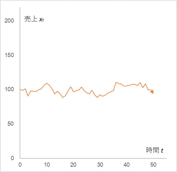
Initial sales x₀=100, sales coefficient α=0.9, constant µ=10, random term ε_t= (probability normal distribution with mean 0 and standard deviation 5)

 

This is the sales trend when there is no COVID-19. Suppose that the corona arrives at t=10 to 13. To reflect this in the calculation, we force the values of the random terms ε₁₀ to ε₁₃ to be large negative values. Now, how will the sales change? See Figure 2.

Figure 2

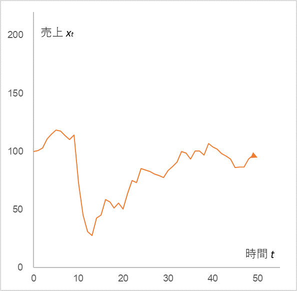
x₀=100, α=0.9. µ=10, ε_t is a random term that follows the same normal distribution as in Figure 1. 

ε₁₀=-40, ε₁₁=-30, ε₁₂=-20, ε₁₃=-10

 

It is true that sales plummeted due to a large negative stimulus between t₁₀ and t₁₃, but what we want you to pay attention to is what happened after that. But what you should pay attention to is what comes after that: the so-called V-shaped recovery. Look at equation (1). We know that sales will increase if the sales coefficient α is greater than 1, but here it is calculated at 0.9. The random term also follows the same probability distribution as in Figure 1 except for t₁₀ to t₁₃. Don’t you think this is very strange?

So, we would like to know the reason why this is so. To make it easier to understand, we will exclude the random term εt from equation (1).

$$x_{t}=αx_{t-1}+µ\tag{2}$$

Incidentally, the random term only plays a role in making the line jagged, so removing it will not change the essential motion. Then, according to Equation (2), let’s examine what actually happens to x₀, x₁, x₂, x₃, … x_n.

$$x_{0}$$

$$x_{1}=αx_{0}+µ$$

$$x_{2}=αx_{1}+µ=α(αx_{0}+µ)+µ=α^2x_{0}+αµ+µ$$

$$x_{3}=αx_{2}+µ=α(α^2x_{0}+αµ+µ)+µ=α^3x_{0}+α~2µ+αµ+µ$$

・

・

・

$$x_{t}=αx_{t-1}+µ=α^tx_{0}+µ(1+α+α^2+α^3+ ・・・+α^t)\tag{3}$$

 

This is where the reason for the mystery finally becomes apparent. This is where the reason for the mystery finally becomes apparent. As time t passes, α^tx₀ approaches zero because α is less than 1. On the other hand, 1+α+α₂+α₃+… +α_t converges to a constant value as shown in Table 1.

Table 1

α	0.9	0.8	0.7	0.6	0.5
1+α+α2+α3+・・・+αt	10.0	5.0	3.3	2.5	2.0

 

From the above, we can see that x_t converges to the value obtained by multiplying 1+α+α²+α³+・・・・・・+α^t in Table 1 by µ. If α = 0.9 and µ = 10, x_t converges to 100, and if α = 0.8 and µ = 10, x_t converges to 50.

By the way, it is interesting to note that the only parameters that determine the convergence value are α and µ, and they do not depend on the initial value x₀. Incidentally, if we change the initial value from 0 to 100 to 200, we get

Figure 3

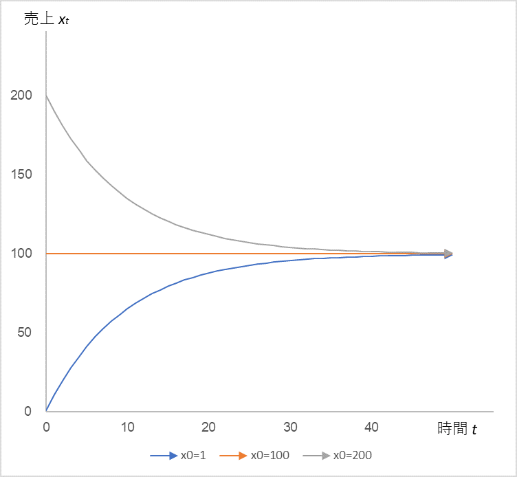
In Equation (2), the time series change of sales x_t when the sales coefficient α = 0.9 and the constant µ = 10 are fixed, and the initial values x₀ = 1, 100, and 200 are used.

 

Indeed, regardless of the initial value, the sales x_t converges to 100. Speaking of convergence, the logistic equation,

$$dx/dt=rx(1-\frac{x}{K})\tag{4}$$

where there is a sense of will to stop growth when x reaches K (see “Growth with an upper bound” in my blog dated May 6, 2021). But at least I don’t sense such a will from the super-simple equation (2), and I couldn’t even predict convergence.

In equation (4), K determines the upper limit, which I assumed to be equivalent to the manager’s perspective. On the other hand, in Equation (2), the combination of α and µ determines the upper bound. Let’s examine the role of these two parameters in more detail.

First, let’s keep µ fixed and move only α.

Figure 4

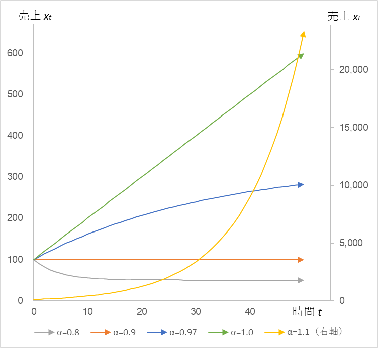
In Equation (2), when x₀ is fixed at 100, µ at 10, and α is set to 0.8, 0.9, 0.97, 1.0, and 1.1, the time series of sales x_t (right axis for α=1.1)

 

We can see that sales x_t is sensitive to α: it converges when α < 1, increases linearly when α = 1, and diverges as an exponential increase when α > 1.

Next, we fix α and move only µ.

Figure 5

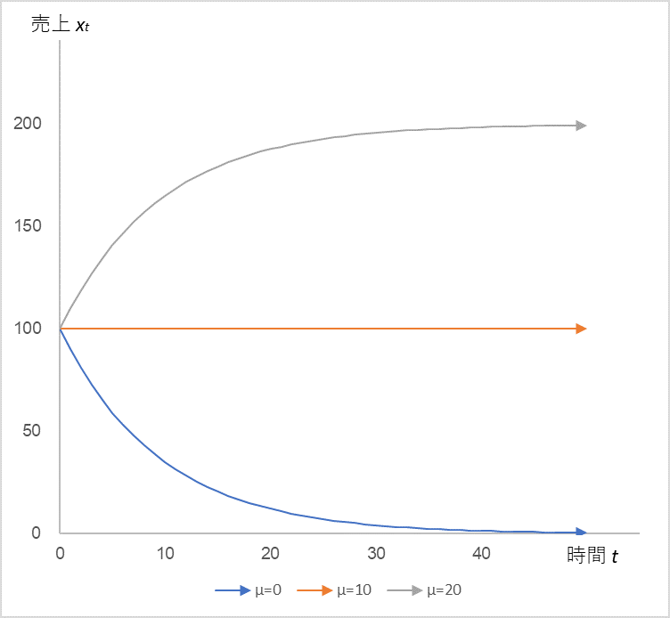
In equation (2), the time series change in sales x_t when x₀=100, α=0.9 is fixed, and µ=0 → 10 → 20

 

Here again, sales x_t is sensitive to µ. Under these assumptions, the manager needs to keep µ above 10 in order to keep sales stable. It is similar in nature to the logistic equation K.

From the above, I came to a very simple conclusion: “Even if you receive a large negative stimulus, if you continue to do what you have been doing, you will always return to your original state.” Moreover, it is backed up by mathematics. This is reassuring. If you refer to the COVID-19 prediction of convergence and manage to get through it with ingenuity and perseverance, you will see a V-shaped recovery in sales. The ingenuity that you have shown during those difficult times will raise the values of α and µ.

The near future is brighter than the past!

If you are interested in the details of the calculation, please refer to Time Series Analysis (1) – Excel.

There will be two more installments in the Time Series Analysis series.

Understanding “Continuity is Power” with Formulas (blog dated September 11, 2021)

The Mathematical Meaning of “Managers Raising Their Eyes” (Blog, September 13, 2021)

 

<Reference>

Tatsuyoshi Okimoto, AR Process, Econometric Time Series Analysis of Economic and Financial Data, Asakura Shoten, 2021

 

The end

 

Back to archive