We have been using the S&P 500, a typical U.S. stock index, to predict stock prices, but today we will use the Nikkei 225. The Excel data can be obtained from the following website.

https://www.macrotrends.net/2593/nikkei-225-index-historical-chart-data

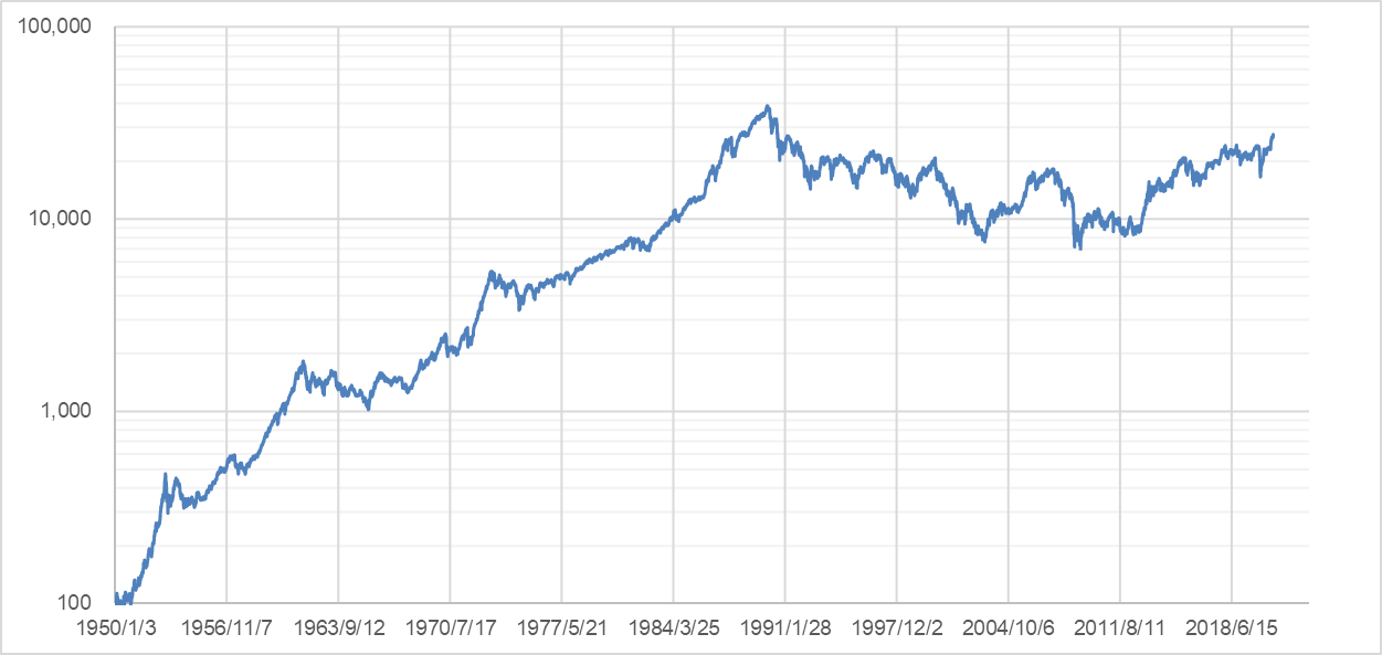
We will use the daily closing prices from January 3, 1950 to December 30, 2020, totaling 17,620. First, let’s chart it to see the movement. The vertical axis is logarithmic.

Figure 0:  Nikkei 225 over the past 71 years

Now, we will use Excel to predict the closing price in 2021.

Step 1)

Focusing on the daily rate of change of the stock price over the past 71 years, classify the number of days of rise and fall and the rate of change of each into the following four patterns

Pattern A:  Number of days of rise > number of days of fall, rise rate > fall rate

Pattern B:  Number of days rising > number of days falling, rate of rise < rate of fall

Pattern C:  Number of days rising < number of days falling, rate of rise > rate of fall

Pattern D:  Number of days rising < number of days falling, rate of rise < rate of fall

Figure 1 shows the number of rising and falling days by year. It can be seen that the number of rising days generally exceeds the number of falling days. Incidentally, over the past 71 years, there have been 9,269 days of upward movement and 8,351 days of downward movement.

Figure 1:  Yearly expression of the number of rising and falling days

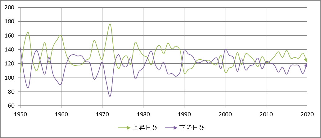
Figure 2 shows the average rate of rise and fall by year. If we look at the linear approximation (dashed line), we can see that the rate of change is increasing with each passing year; the average rate of change since 1950 is 0.831% for the rise and 0.847% for the fall, with the fall rate slightly exceeding the rise rate.

Figure 2:  Average rate of increase and average rate of decrease by year

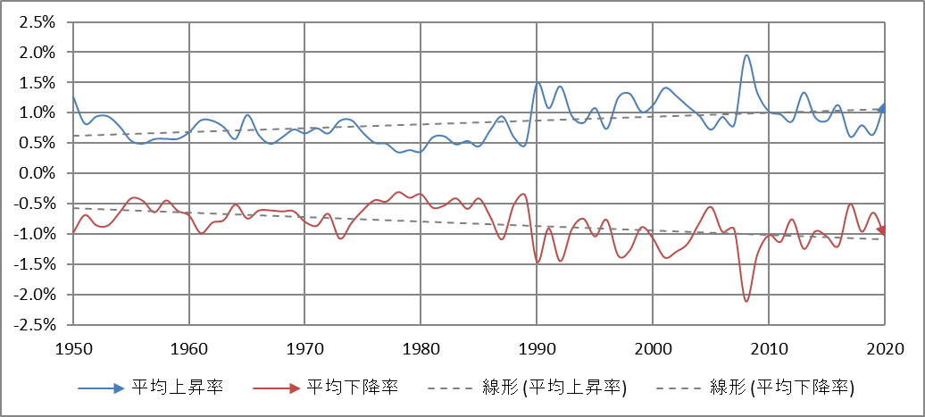
Table 1 shows the changes over the past 71 years, categorized by the four patterns.

Table 1:  Classification of expression patterns over the past 71 years

Pattern	Number of occurrences	Average rate or rise	Average rate of fall	Average number of days of rise	Average number of days of fall
A	22	0.739%	-0.669%	135	114
B	24	0.815%	-0.886%	132	106
C	19	0.905%	-0.843%	122	127
D	6	1.154%	-1.195%	118	129

 

Step 2)

Next, calculate the stock price to be reached at the end of 2021 for each pattern using the formula for stock price prediction.

<Formula for predicting the stock price $x_{0}$ in $n$ days>

$$x_{n}=x_{0} (1 + a)^p(1 – b)^q$$

$$(p + q = n, a, b > 0)$$.

where $x_{0}$ is the initial value; if the forecast is for the closing price in 2021, the initial value should be 27,444.17 yen, the value of the closing price in 2020. Let $a$ be the average rate of increase, $b$ the average rate of decrease, $p$ the number of days of increase, and $q$ the number of days of decrease.

For the derivation of the formula for stock price prediction, see “How accurate is the prediction of stock price one year from now? for more details.

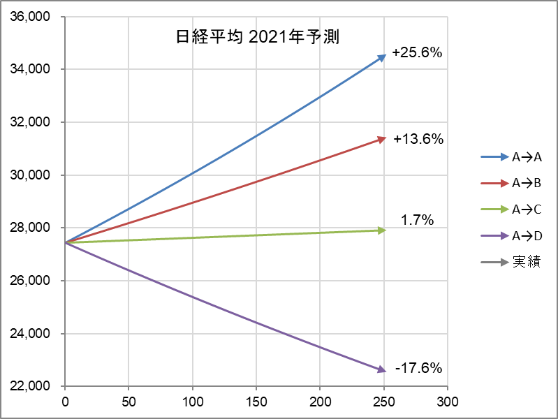
Table 2 shows the result of the calculation using the data in Table 1. For example, there is a 38.1% probability that Pattern A will continue next year, in which case the closing price will be 34,473.60 yen (an increase of 25.6% over the previous year).

Table 2:  Closing prices for 2021 predicted using the prediction formula

Transition pattern	Number of occurrences	Probability of occurrence	Forecast for closing price in 2021	Change
A → A	8	38.1%	34,470.60	25.6%
A → B	6	28.6%	31,187.36	13.6%
A → C	6	28.6%	27,899.03	1.7%
A → D	1	4.8%	22,627.41	-17.6%
	21	100.0%

 

Figure 3 is a graphical representation of Table 2.

Figure 3:  Forecast by pattern at the end of 2021

 

Step 3)

Finally, we check the above predictions against the probability distribution obtained by the other calculation method. While the stock price tries to increase exponentially, it always fluctuates up and down. The formula for this is

$$frac{dx}{dt}=rx+vxfrac{dB(t)}{dt}$$.

The result is where $x$ is the stock price, $r$ is the growth coefficient, $v$ is the fluctuation coefficient, and $B(t)$ is the daily random change. This equation represents the moment-to-moment changes in the stock price $x$. The accumulation of these changes is the trajectory of the stock price (the chart in Figure 0). The above equation is called a stochastic differential equation, and the calculation of the accumulation is called solving (integrating) the differential equation. The result is.

$$x=x_{0} e^{(r-frac{v^2}{2})t+vB(t)}$$.

When the time has passed by t The equation tells us how much the stock price will be when time elapses by t. $x_{0}$ is the initial value. For more information on how to determine $r$ (growth coefficient), $v$ (fluctuation coefficient), and $B(t)$ (daily change), please see my April 21, 2020 blog, “When will the stock market recover from the Corona shock? for more details. All calculations can be done in Excel.

Figure 4 shows the probabilistic distribution of the stock price when the initial value is the closing price in 2020. The orange line $µ$ is the center of the probability distribution, and the dashed lines indicate +1σ, -1σ, +2σ, -2σ…$. The probability of falling into the range decreases as the number increases. Then, superimpose the four predictions above. We can see that they are all within the range of $pm 1σ$, and there is no contradiction.

Figure 4:  Probability distribution of Nikkei 225 and prediction of closing price at the end of 2021

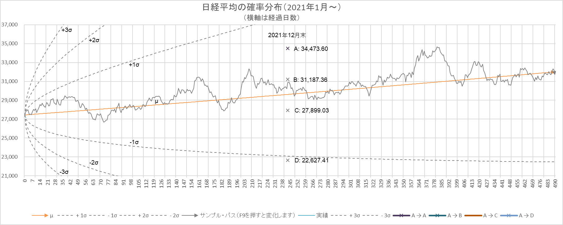
The gray line is a sample path.

The above is the forecast calculation. We will now check the predictions against the actual Nikkei 225 in 2021, so stay tuned!

 

Back to archive